Reading this paper for GSOC 2025 - CERN.

This paper focuses on data manipulations prior to using a compression algorithm. The highlight are two data preprocessing algorithms - Addition and Multiplication. Employing these algorithms improve the compressor effectiveness by increasing the number of bit values shared in the dataset to reduce its entropy. This objective is also part of the preprocessing method proposed by Kl¨ower et al. in Nature Computational Science 1 , which is used as benchmark for the evaluation of the proposed techniques.

Background

• Floating point numbers

1) Sign ‘S’: {s1} bit. ‘0’ for n ≥ 0, ‘1’ for n < 0.
2) Exponent ‘E’: {e1 . . . e8} bits. It is biased, meaning that it is interpreted as an unsigned integer once the bias b = 2k−1 − 1 = 127 is subtracted from it, where k is the number of exponent bits.
3) Mantissa ‘M’: {m1 . . . mi . . . m23} bits. Each mi represents 2E−b−i \

In order to translate bits to numbers, we use the equations n = (−1)S · 2 E−b · (1 + M · 2 −23) = (−1)S · [2EU + m1 · 2 EU −1 + · · · + m23 · 2 EU −23]

Since the distance between two consecutive FP-representable numbers depends on their exponent, i.e. EU , the further we go from zero, the sparser floating point numbers become on the real axis, as per

Algorithm

Addition

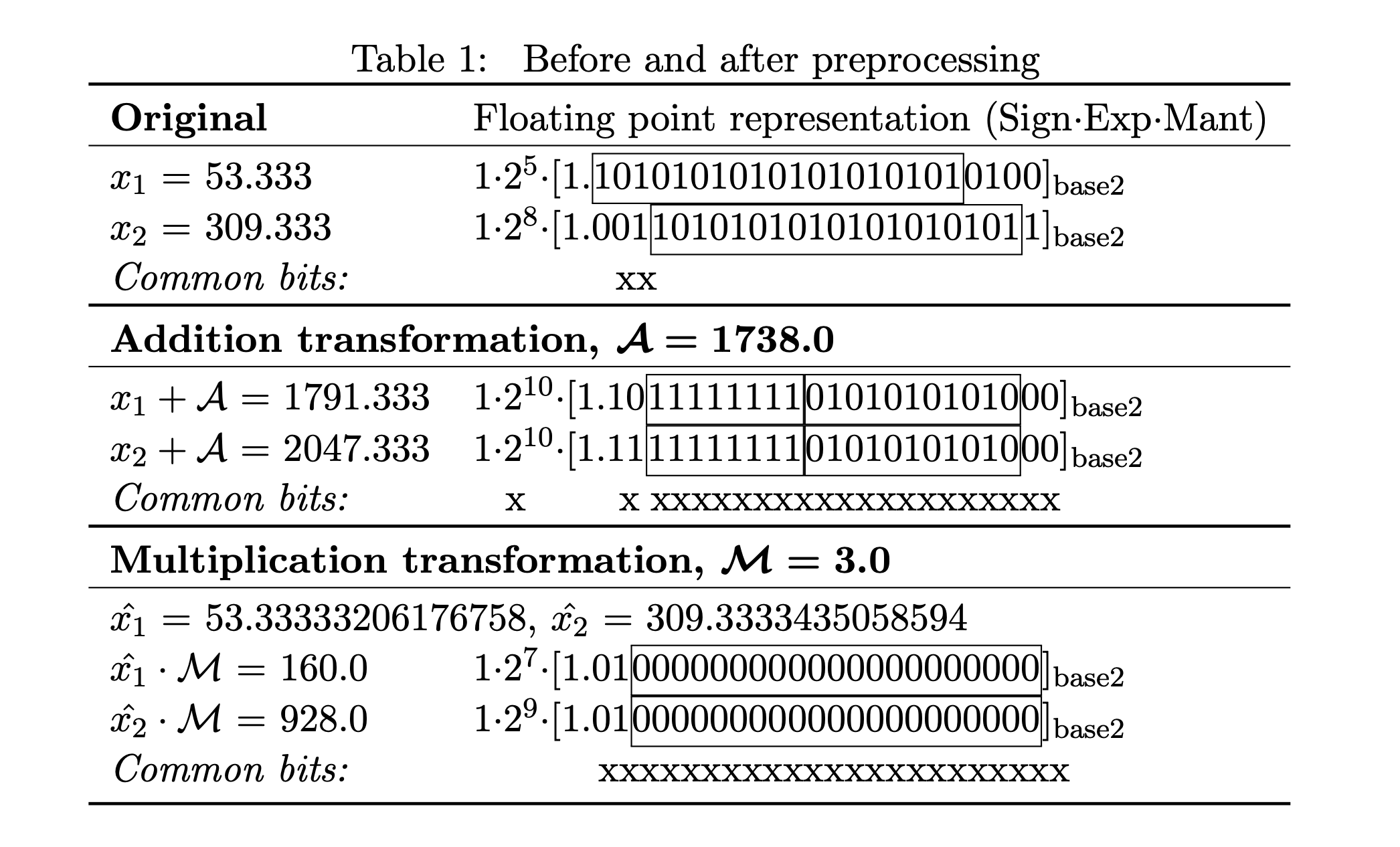
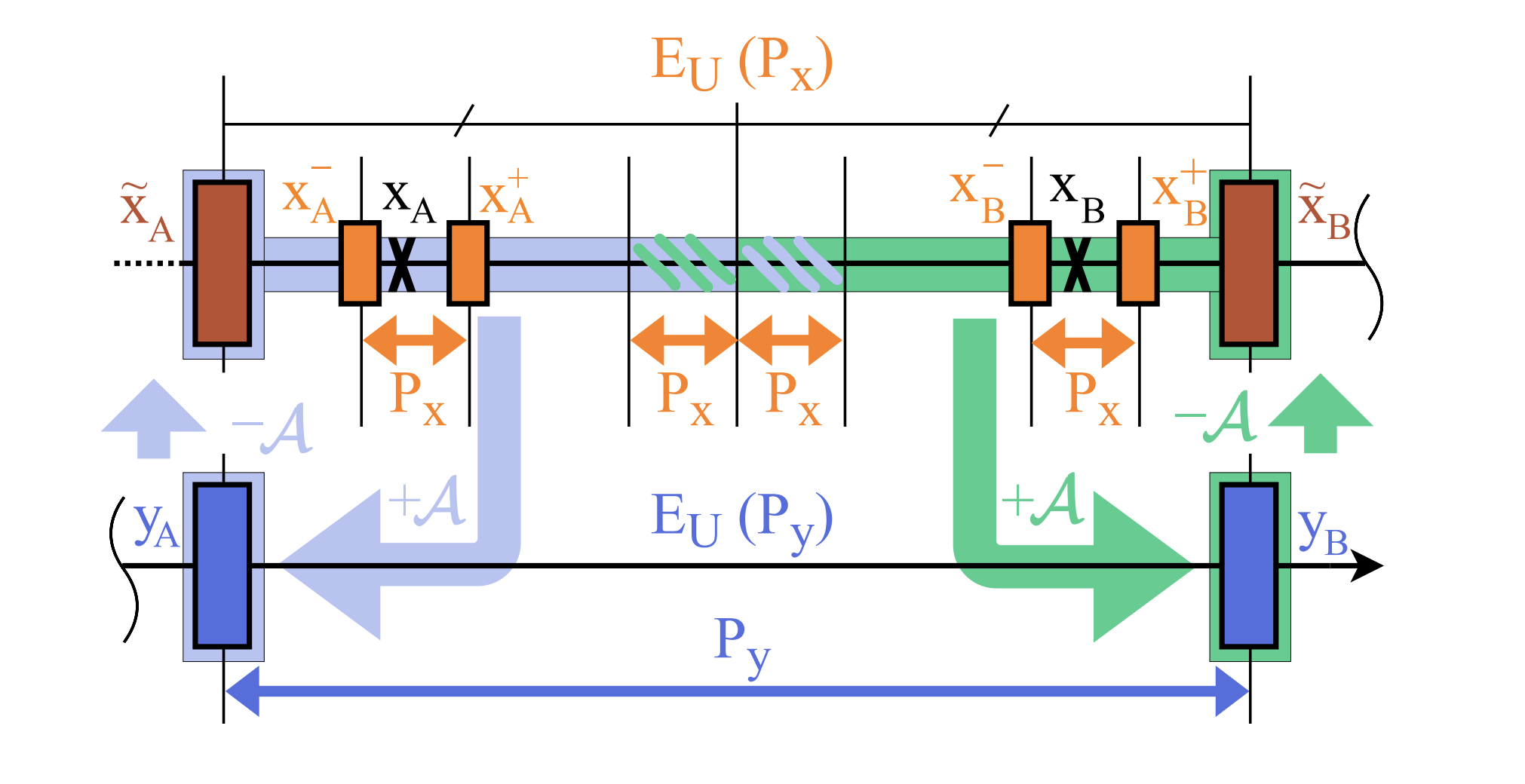
This method can be summarized as the following operation: yi = xi + A, ∀xi ∈ D (7) where A > 0 is called addition parameter, D is the dataset. The idea is to shift all samples of the dataset to a suitable region on the real axis. As illustrated in Fig. 4, by strategically choosing A we can guarantee that all numbers in dataset after the addition transform share the exponent and several mantissa bits. The cost is a possible recovery error due to changing precision from the original region of each sample xi to the new yi ’s precision. In order to recover the original data, we apply the inverse transformation ˜xi = yi − A, thus A needs to be stored as metadata.

Recovery Error in Addition

By applying the inverse transform for recovering the sample, we obtain ˜xA = yA − A. Both ˜xA and ˜xB belong to the subset of numbers in the Px region having no component smaller than Py, since they have at least log2 ( Py Px ) zeros in the least significant portion of the mantissa. Supposing that all samples after being transformed have the same EU (Py), ˜xA and ˜xB will be approximating every xi such that x˜A ≤ xi ≤ x˜B. This is because given xi ∈ D, during the addition transform yi = xi + A, we are losing any info smaller than Py, and with ˜xi = yi − A we are filling the mantissa bits we lost with zeros. Therefore, xi + A = yA, x˜A = yA − A ∀xi ∈ [˜xA; ˜xA + Py/2 − Px] xj + A = yB, x˜B = yB − A ∀xj ∈ [˜xA + Py/2 + Px; ˜xB] (8) meaning that different numbers belonging to the same precision region will result in different recovery errors. Due to the standard, yi and ˜xi for xi ∈˜xA +Py/2−Px; ˜xA +Py/2+Px depend on the rounding method and the selected A. The use of the addition transform ensures a bound in the recovery error, which is a function of Py ∆ ≤ 2 E y U −23−1 = Py 2 , (9) where E y U is the unbiased exponent shared by all samples after the transform.

a. it is as large as possible while keeping ∆ and δ within the user requirements and complying with b) and c);
b. the transformed dataset is aligned with the largest powers of 2 in the region;
c. it has the same precision of the numbers resulting from the addition with A \

Select A : max(xi ∈ D) + A = 2EA U +1 − 2 EA U −23

Multiplication

This method can be summarized as

yi = ˆxi

· M, xˆi = f(xi

,M) ∀xi

xi ∈ D (11) where we call M the multiplication parameter, and f is a function that substitutes each data sample xi in the dataset with ˆxi , a version arbitrarily close to the original, but with the nice property of resulting in many zeros once multiplied by M. So, in contrast to the addition transform, we apply the multiplication transform on ˆxi rather than on the original xi . We aim to maximize the number of least significant bits in the mantissa equal to zeros. Let us explain this with an example

We consider x1 = 363.754 and x2 = 366, with x2 having 16 consecutive zeros at the end of the mantissa and x1 having none. In order to increase the number of common ending zeros, we propose substituting x1 and x2 with numbers that show the desired zeros after being multiplied by a carefully selected 6 multiplication parameter M. We consider ˆx1 = 363.7894592285156 and ˆx2 = 366.03509521484375 with M = 57. Then, y1 = ˆx1 ·M = 20736.0 and y2 = ˆx2 ·M = 20864.0, which share the last 16 zeros. By storing y1, y2 and M, we can recover the original numbers via the divisions ˜x1 = y1/M = ˆx1 and ˜x2 = y2/M = ˆx2 with maximum deviation δ < 0.01%. Other existing methods, like , directly approximate x1 by removing all unwanted least significant mantissa bits to reach 16 ending zeros, where the recovered sample is ˜x1 = 362.0, with deviation δ = 0.48%.

• Patterns are bit-shifting invariant.
• Starting patching from the left results in a larger error and more common zeros.
• Typically, the more bits you modify from the original mantissa, the bigger the error will be.
• More zeros at the end of the mantissa do not necessarily mean a larger recovery error.

Performance Evaluation

For all datasets and compressors, with ∆ ≤ 1 or δ ≤ 1%, both addition and multiplication transforms improve compression with respect to the non-preprocessed datasets, with reductions upto 80%
We also notice that when addition and multiplication transforms outperform the non-preprocessed datasets