DPO v/s PPO v/s GRPO

In order to understand what these fancy “alignement” algorithms mean, let’s go back to the basics first - RLHF. There are many applications such as writing stories where you want creativity, pieces of informative text which should be truthful, or code snippets that we want to be executable.

Writing a loss function to capture these attributes seems intractable and most language models are still trained with a simple next token prediction loss (e.g. cross entropy). To compensate for the shortcomings of the loss itself people define metrics that are designed to better capture human preferences such as BLEU(bilingual evaluation understudy is an algorithm for evaluating the quality of text which has been machine-translated from one natural language to another) or ROUGE(Recall-Oriented Understudy for Gisting Evaluation, is a set of metrics and a software package used for evaluating automatic summarization and machine translation software in natural language processing.). While being better suited than the loss function itself at measuring performance these metrics simply compare generated text to references with simple rules and are thus also limited.

A brief intro to RLHF

As a starting point RLHF use a language model that has already been pretrained with the classical pretraining objectives. OpenAI (InstructGPT) , Deepmind(Gopher)

Pretraining
Core to starting the RLHF process is having a model that responds well to diverse instructions. With a language model, one needs to generate data to train a reward model, which is how human preferences are integrated into the system.

Reward model training
Generating a reward model (RM, also referred to as a preference model) calibrated with human preferences is where the relatively new research in RLHF begins. The underlying goal is to get a model or system that takes in a sequence of text, and returns a scalar reward which should numerically represent the human preference. The system can be an end-to-end LM, or a modular system outputting a reward (e.g. a model ranks outputs, and the ranking is converted to reward). The output being a scalar reward is crucial for existing RL algorithms being integrated seamlessly later in the RLHF process.

These LMs for reward modeling can be both another fine-tuned LM or a LM trained from scratch on the preference data. For example, Anthropic has used a specialized method of fine-tuning to initialize these models after pretraining (preference model pretraining, PMP) because they found it to be more sample efficient than fine-tuning, but no one base model is considered the clear best choice for reward models.

These LMs for reward modeling can be both another fine-tuned LM or a LM trained from scratch on the preference data. For example, Anthropic has used a specialized method of fine-tuning to initialize these models after pretraining (preference model pretraining, PMP) because they found it to be more sample efficient than fine-tuning, but no one base model is considered the clear best choice for reward models.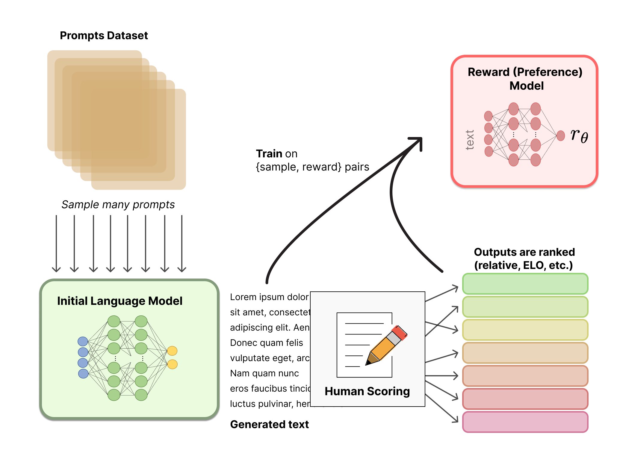

Finetuning with RL
Here comes the policies. Let’s first formulate this fine-tuning task as a RL problem. First, the policy is a language model that takes in a prompt and returns a sequence of text (or just probability distributions over text). The action space of this policy is all the tokens corresponding to the vocabulary of the language model (often on the order of 50k tokens) and the observation space is the distribution of possible input token sequences, which is also quite large given previous uses of RL (the dimension is approximately the size of vocabulary ^ length of the input token sequence). The reward function is a combination of the preference model and a constraint on policy shift.

The reward function is where the system combines all of the models we have discussed into one RLHF process. Given a prompt, x, from the dataset, the text y is generated by the current iteration of the fine-tuned policy. Concatenated with the original prompt, that text is passed to the preference model, which returns a scalar notion of “preferability”, r θ r θ ​ . In addition, per-token probability distributions from the RL policy are compared to the ones from the initial model to compute a penalty on the difference between them.

Kullback–Leibler (KL) Divergence

In mathematical statistics, the Kullback–Leibler (KL) divergence (also called relative entropy and I-divergence), denoted as
D_KL(P ∥ Q), is a type of statistical distance: a measure of how much a model probability distribution Q differs from a true probability distribution P.

Mathematically, it is defined as:

D_KL(P ∥ Q) = Σ P(x) * log(P(x) / Q(x))

where the sum is taken over all possible values x in the set X.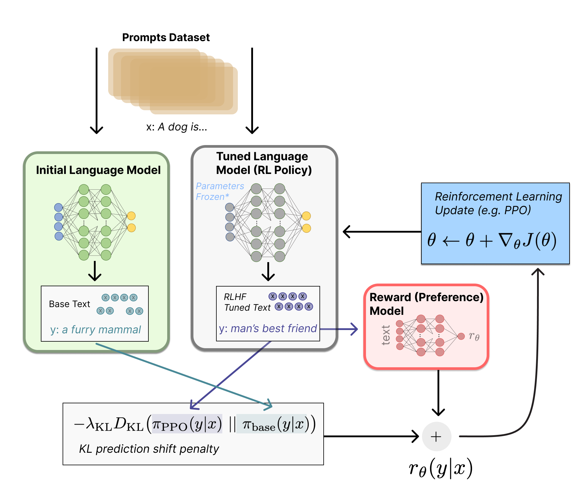

PPO - Proximal Policy Optimization (On-policy)

• Policy
• Reward Model
• Calue Function
  1. Generate Text (Rollout)
  2. Get Score (Reward Model)
  3. Calculate Advantage (Generalized Advantage Estimation)
  4. Optimize the LLM (Policy Update)
     — Encourages higher rewards: It pushes the LLM to generate text that gets higher scores. — Limits policy changes (Clipped Surrogate Objective): It prevents the policy from changing too much in one update, ensuring stability.
     — KL Divergence Penalty: It adds a penalty if the new policy deviates too far from the old policy, further enhancing stability.
     — Entropy Bonus: It also includes an entropy bonus. Entropy, in simple terms, measures how “random” or “diverse” the LLM’s text generation is. Adding an entropy bonus encourages the LLM to be a bit more exploratory and less “stuck in a rut” of always generating the same, predictable responses. It helps prevent the LLM from becoming too “certain” too quickly and missing out on potentially better strategies.
  5. Update the Value Function (Critic Update)

def ppo_loss_with_gae_entropy(old_policy_logprobs, new_policy_logprobs, advantages, kl_penalty_coef, clip_epsilon, entropy_bonus_coef):
   
    ratio = np.exp(new_policy_logprobs - old_policy_logprobs) # Probability Ratio

    # Clipped Surrogate Objective (limit policy change)
    surrogate_objective = np.minimum(ratio * advantages, np.clip(ratio, 1-clip_epsilon, 1+clip_epsilon) * advantages)
    policy_loss = -np.mean(surrogate_objective)

    # KL Divergence Penalty (stay close to old policy)
    kl_divergence = np.mean(new_policy_logprobs - old_policy_logprobs)
    kl_penalty = kl_penalty_coef * kl_divergence

    # Entropy Bonus (encourage exploration)
    entropy = -np.mean(new_policy_logprobs) # Simplified entropy (higher prob = lower entropy, negate to maximize entropy)
    entropy_bonus = entropy_bonus_coef * entropy

    total_loss = policy_loss + kl_penalty - entropy_bonus # Subtract entropy bonus as we want to *maximize* entropy
    return total_loss

DPO - Direct Preference Optimization (Off-policy)

• Direct to the Point
• DPO — No RL Loop, Just Preferences (Clever loss function with human GT)

1) Preference Data 2) Direct Policy Update (very similar to a binary cross-entropy loss) 3) Stay Close to the Reference Model (Implicit KL Control)

def dpo_loss(policy_logits_preferred, policy_logits_dispreferred, ref_logits_preferred, ref_logits_dispreferred, beta_kl):
    """Conceptual DPO Loss (simplified - directly using logits)."""

    # 1. Get log probabilities from logits (for preferred and dispreferred responses, current and reference models)
    policy_logprob_preferred = F.log_softmax(policy_logits_preferred, dim=-1).gather(...) # Extract log prob of actual tokens in preferred response
    policy_logprob_dispreferred = F.log_softmax(policy_logits_dispreferred, dim=-1).gather(...) # Extract log prob of actual tokens in dispreferred response
    ref_policy_logprob_preferred = F.log_softmax(ref_logits_preferred, dim=-1).gather(...) # Same for reference model
    ref_policy_logprob_dispreferred = F.log_softmax(ref_logits_dispreferred, dim=-1).gather(...)

    # 2. Calculate log ratio (using log probabilities - as before)
    log_ratio = policy_logprob_preferred - policy_logprob_dispreferred - (ref_policy_logprob_preferred - ref_policy_logprob_dispreferred)

    # 3. Probability of preference (Bradley-Terry Model - implicit reward signal)
    preference_prob = 1 / (1 + np.exp(-beta_kl * log_ratio))

    # 4. Binary Cross-Entropy Loss (optimize policy directly)
    dpo_loss = -np.log(preference_prob + 1e-8)
    return dpo_loss

GRPO - Group Relative Policy Optimization (On-policy)

GRPO’s Trick: Group-Based Advantage Estimation (GRAE): GRPO’s magic ingredient is how it estimates advantages. Instead of a critic, it uses a group of LLM-generated responses for the same prompt to estimate “how good” each response is relative to the others in the group. 1) Generate a Group of Responses 2) Score the Group (Reward Model) 3) Calculate Group Relative Advantages (GRAE — Comparing Within the Group) 4) Optimize Policy (PPO-like Objective with GRAE)

def grae_advantages(rewards):
    """Conceptual Group Relative Advantage Estimation (Outcome Supervision)."""
    mean_reward = np.mean(rewards)
    std_reward = np.std(rewards)
    normalized_rewards = (rewards - mean_reward) / (std_reward + 1e-8)
    advantages = normalized_rewards # For outcome supervision, advantage = normalized reward
    return advantages


def grpo_loss(old_policy_logprobs_group, new_policy_logprobs_group, group_advantages, kl_penalty_coef, clip_epsilon):
    """Conceptual GRPO Loss (averaged over a group of responses)."""
    group_loss = 0
    for i in range(len(group_advantages)): # Iterate over responses in the group
        advantage = group_advantages[i]
        new_policy_logprob = new_policy_logprobs_group[i]
        old_policy_logprob = old_policy_logprobs_group[i]

        ratio = np.exp(new_policy_logprob - old_policy_logprob)
        clipped_ratio = np.clip(ratio, 1 - clip_epsilon, 1 + clip_epsilon)
        surrogate_objective = np.minimum(ratio * advantage, clipped_ratio * advantage)
        policy_loss = -surrogate_objective

        kl_divergence = new_policy_logprob - old_policy_logprob
        kl_penalty = kl_penalty_coef * kl_divergence
        group_loss += (policy_loss + kl_penalty) # Accumulate loss for each response in group

    return group_loss / len(group_advantages) # Average loss over the group

It’s not about fancy generation - Chain of Thought

Incorporating preference learning with CoT produces more accurate results. (Obviously!)

My opinions

Personally, I had prophesised that key to intelligence is RL. Intelligence in itself is subjective product of agent-environment interactions. It is only intuitive that modelling such systems can be rewarding (No pun intended).

References

https://huggingface.co/blog/rlhf
https://anukriti-ranjan.medium.com/preference-tuning-llms-ppo-dpo-grpo-a-simple-guide-135765c87090
https://huggingface.co/blog/NormalUhr/rlhf-pipeline